Pipelined Execution#
On the Cerebras Wafer Scale Engine (WSE) you can run neural networks of sizes ranging from extremely large, such as a GPT-3 model, to smaller-sized models, such as BERT. While model sizes varies widely, the capacity of an accelerator is limited, and the largest models cannot fit into that memory. We therefore support two execution modes, one for models of some limited size, and one for models of arbitrary size.
Note
In the Original Cerebras Installation, only pipelined execution mode is supported. If you want to learn more about Weight Streaming mode to train neural network models above 1 billion parameters, visit Concepts and Guides
The execution mode refers to how the Cerebras runtime loads your neural network model onto the Cerebras Wafer Scale Engine (WSE). The execution mode supported in the Original Cerebras Installation is :
Pipelined (or Layer Pipelined): In this mode, all the layers of the network are loaded altogether onto the Cerebras WSE. This mode is selected for neural network models below 1 billion parameters, which can fit enirely in the on-chip memory.
Layer pipelined computation#
The rest of this section provides a high-level understanding of these this execution mode using a simple FC-MNIST network as an example.
Example neural network#
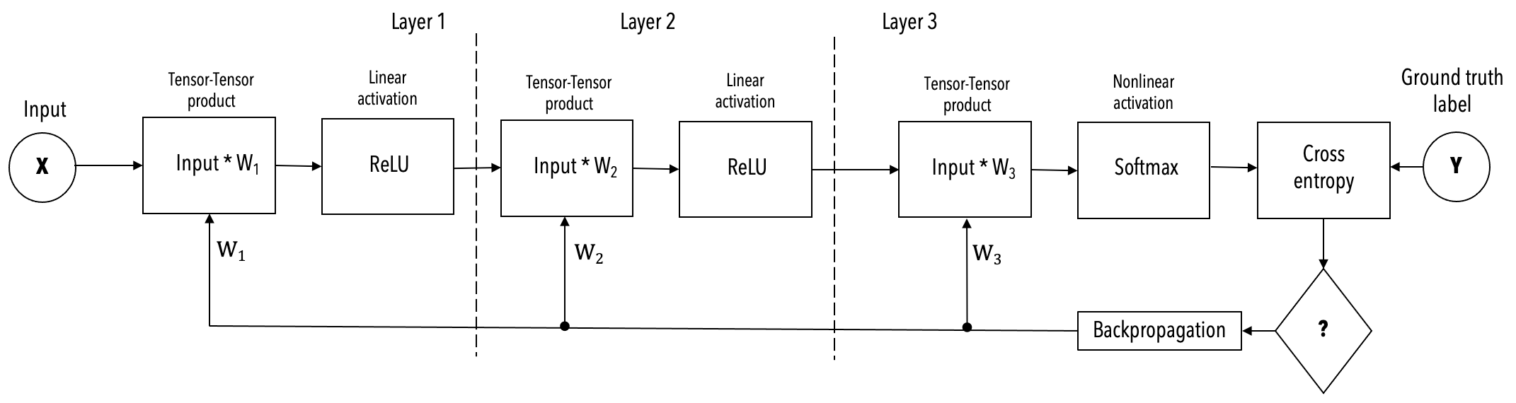
The simplified example, shown below, of a 3-layer FC-MNIST network is used in the following description of the execution mode.
Layer pipelined mode#
The layer pipelined execution mode works like this:
Training job is launched from the chief node. The training job is divided in compilation and execution.
During compilation in the chief node
The Cerebras compiler extracts the graph of operations from your code in PyTorch or TensorFlow and maps to the supported kernels in the Cerebras Software Platform. A mathematical representation of these layers is shown in
cs-exec-mode-fcmnist-math-original. If you are interested in this lightweight compilation, you can use the flagvalidate_only
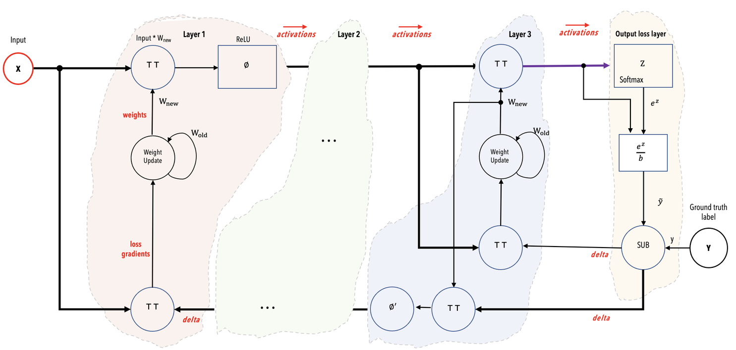
Mathematical representation of example network showing color-coded layers and the activations flowing from one layer to the next layer.#
The Cerebras compiler maps each kernel/layer of the network onto a region (a rectangle) of the Cerebras WSE. It connects the regions with data paths to allow activations and gradients to flow from layer to layer. It chooses sizes of regions and places them so as to optimize the throughput, which is the number of training samples that the wafer can accept per unit time. If you are interested in doing precompilation, you can use the flag
--compile_only.
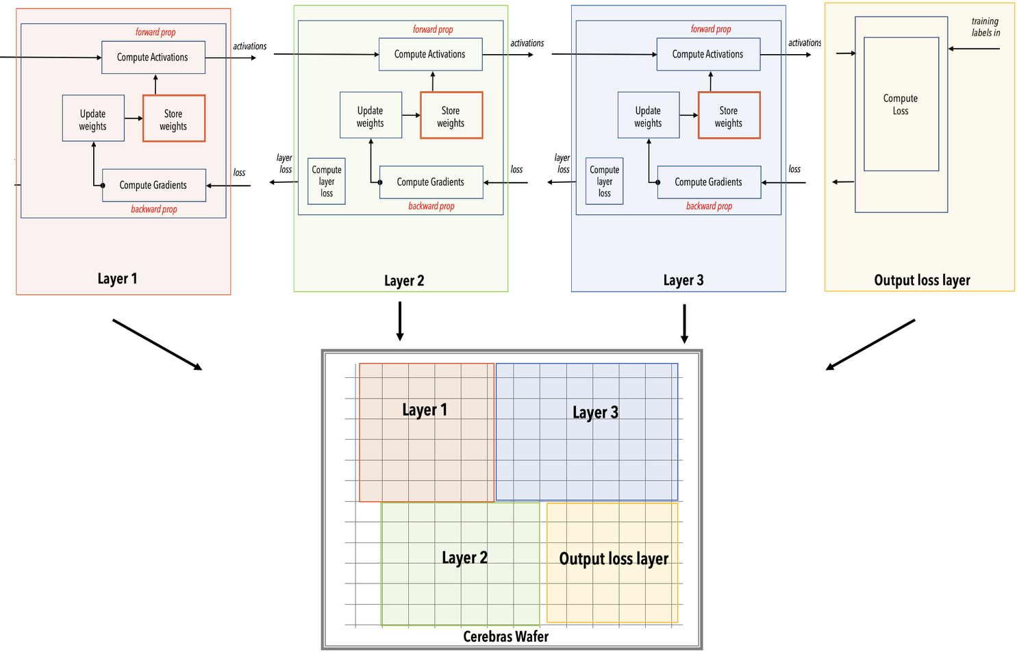
Layer pipelined mapping. Notice that all the layers reside on the WSE all the time. This is an example on how the color-coded parts of the WSE mapped into the network.#
The entire network is loaded onto the Cerebras WSE inside the CS-2 system.
Training starts:
In the worker nodes, training data is processed into samples and then stremed to the WSE inside the CS-2 system.
In the WSE, As shown in
cs-exec-mode-layerpipe-execution-originalData samples are received and processed in the input layer. As soon as the input layer finishes with a minibatch, it requests the next minibatch of training data.
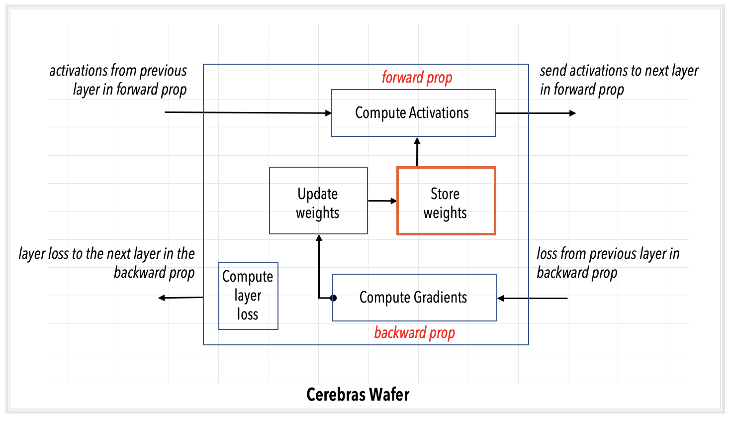
Activations pass from layer to subsequent layer for forward prop.
After the loss and initial gradient layer are computed, activation gradients flow from layer to previous layer for backprop.
Weights are updated on the WSE at the end of each backprop step. The weights remain in the memory of the WSE region assigned by the compiler to that layer.
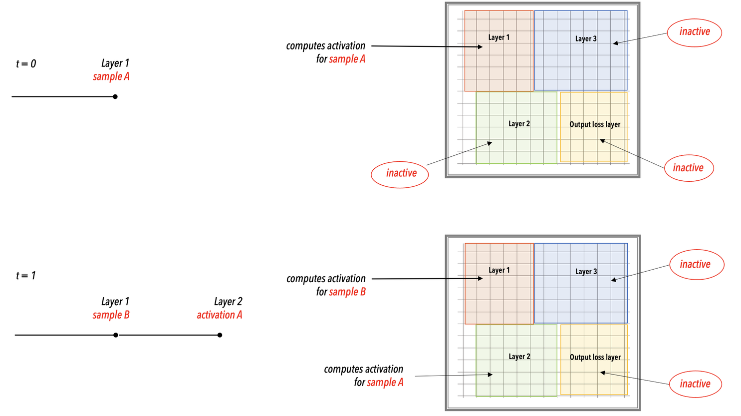
Layer pipeline execution. In the layer pipelined execution, there is an initial latency period after which all the layers of the network enter a steady state of active execution. In this illustration, the network enters the steady state of execution at step 3 and thereafter.#
In the chief node,
As loss values are computed on the WSE, they are streamed to the user node.
At specified intervals, all the weights can be downloaded to the chief node to save checkpoints.