Weight Streaming and Pipelined Execution#
On the Cerebras Wafer-Scale Engine (WSE) you can run neural networks of sizes ranging from extremely large, such as a GPT-3 model, to smaller-sized models, such as BERT. While model sizes varies widely, the capacity of an accelerator is limited, and the largest models cannot fit into that memory. We therefore support two execution modes, one for models of some limited size, and one for models of arbitrary size.
The execution mode refers to how the Cerebras runtime loads your neural network model onto the Cerebras Wafer-Scale Engine (WSE). Two execution modes are supported:
Weight streaming mode: In this mode, one layer of the neural network model is loaded at a time. This layer-by-layer mode is used to run large models, models for which one layer’s weights fit in memory, but the whole model’s do not.

Fig. 2 Weight streaming mode#
Layer pipelined mode: In this mode, all the layers of the network are loaded altogether onto the Cerebras WSE. This mode is selected for neural network models below one billion parameters, which can fit entirely in the on-chip memory.
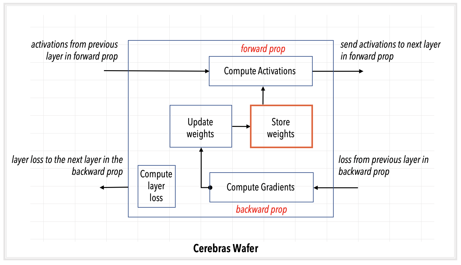
Fig. 3 Layer pipelined mode#
The rest of this section explains these modes, using an FC-MNIST network as an example.
Example neural network#
The example shown below, of a 3-layer FC-MNIST network, is used to explain the two execution modes.
Weight streaming mode#
The weight streaming execution mode is used for extremely large neural network models and for networks with very large input sizes. In the weight streaming execution mode, the network is loaded layer by layer onto the WSE.
At runtime, one layer is loaded onto the WSE at each step, as shown in Fig. 4. A single layer is executed each step. In forward prop, the weights are streamed from the MemoryX server to the WSE. In backprop, the weights are again streamed from MemoryX to the WSE, weight gradients are computed on the WSE then streamed from the WSE to MemoryX for storage and for learning, in which the weights are adjusted using the weight gradient and the learning algorithm.

Fig. 4 Weight streaming execution mode.#
The weight streaming execution mode works like this (using the FC-MNIST example). Recall that the user launches first a compilation and then an execution job.
During the compilation job:
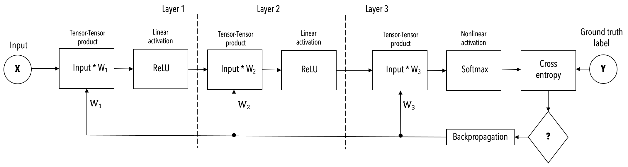
The Cerebras compiler extracts the graph of operations from the code and maps the operations to the supported kernels of the Cerebras Software Platform. Each such matched kernel constitutes a layer in the network dataflow graph. A mathematical representation of these layers is shown in Fig. 7. If you are interested in seeing the result of this lightweight phase of compilation, you can use the
--validate_onlyflag.The Cerebras compiler plans the mapping of one kernel/layer at a time to the whole WSE, first for the forward, then for the backward prop passes. If multiple CS-2 systems are requested in the Cerebras Wafer-Scale cluster, then for every layer, the same mapping is used across for all CS-2 systems. If you are interested in doing precompilation, you can use the
--compile_onlyflag.
Training starts:
Forward propagation, as shown in Fig. 5
Layer 1 is loaded onto the WSE first. Input pre-processing servers process and stream training data to the WSE. MemoryX streams layer 1’s weights into the WSE. If multiple CS-2s are requested in the training job, SwarmX broadcasts the weights from MemoryX to the WSEs. The batch of training samples is sharded into equally large subsets of training examples, with one shard going to each of the CS-2s. This technique is known as data parallelism.
Each WSE, in parallel with the others, performs the layer 1 forward computation.
The computed activations for layer 1 remain in WSE memory.
Next, MemoryX broadcasts the weights of layer 2 to the WSEs.
Each WSE performs the layer 2 forward computations using its stored layer 1 activations.
The same again for layer 3.
In this manner, the forward compute for each layer is performed by using the stored computed activations of the prior layer. The computed activations of the current layer, in turn, are stored on the WSE memory to be used by the next layer that is loaded.
At the loss layer, the ground truth labels from the training data are used to compute the network loss delta, which is the gradient of the scalar loss with respect to the output layer (layer 3) activation. This loss delta is used to compute layer by layer deltas and weight gradients during the backward pass.

Fig. 5 Schematic representation of the forward propagation in Weight Streaming mode.#
Backward propagation, as shown in Fig. 6
The layer 3 weights are broadcast from the MemoryX to WSEs, which perform the gradient and delta computations for layer 3. (The implementation can, of course, retain the weights of this, the output layer, to save time.
The layer 3 gradients are streamed out of the WSE to the SwarmX , which reduces (adds together) the weights from the multiple WSEs and presents their sum to MemoryX. Then MemoryX uses the aggregate gradient in the learning algorithm to update its stored copy of the layer weights.
Next, the layer 2 weights are streamed from the MemoryX to the WSE, and the WSE similarly performs the gradient and delta computations for the layer 2. The layer 2 gradients are then streamed out of the WSE to the MemoryX where weight updates occur. If multiple CS-2s are requested in the training job, SwarmX broadcasts the weights from the MemoryX to the WSEs and reduces the gradient updates from the WSEs to the MemoryX.
The backward pass continues in this manner until layer 1 gradients are streamed out to the MemoryX where the weights are updated and the forward pass for the next training batch begins with the updated weights.

Fig. 6 Schematic representation of the backward propagation in Weight Streaming mode.#
Meanwhile, in the user node,
As loss values are computed on the WSEs, they are reduced by SwarmX and sent to the user node.
At specified intervals, all the weights can be downloaded from MemoryX to the user node to save checkpoints.
Layer pipelined mode#
In layer pipelined mode, the entire model, all the weights, resides at all times in the WSE of the one CS-2 used. As always, the user launches a compilation and an execution job from the user node:
Training job is launched from the user node. To jobs are submited to the management node in the Cerebras cluster: a compilation job and an execution job.
During the compilation job:
o The Cerebras compiler extracts the graph of operations from the code and maps the operations to the supported kernels of the Cerebras Software Platform. Each such matched kernel constitutes a layer in the network dataflow graph. A mathematical representation of these layers is shown in Fig. 7. If you are interested in seeing the result of this lightweight phase of compilation, you can use the
--validate_onlyflag.
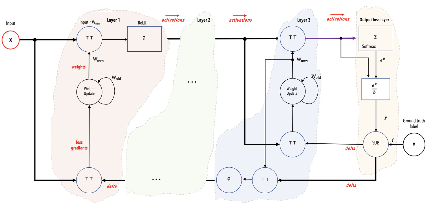
Fig. 7 Mathematical representation of example network showing color-coded layers and the activations flowing from one layer to the next layer.#
The Cerebras compiler maps each kernel/layer of the network onto a region (a rectangle) of the Cerebras WSE. It connects the regions with data paths to allow activations and gradients to flow from layer to layer. It chooses sizes of regions and places them so as to optimize the throughput, which is the number of training samples that the wafer can accept per unit time. If you are interested in doing precompilation, you can use the
--compile_onlyflag.
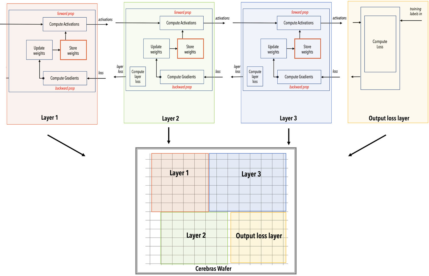
Fig. 8 Layer pipelined mapping. Notice that all the layers reside on the WSE all the time. This is an example on how the color-coded parts of the WSE mapped into the network.#
The entire network is loaded onto the Cerebras WSE inside the CS-2 system.
Training starts:
In the input pre-processing servers, training data is processed into samples and then streamed to the WSE inside the CS-2 system.
In the WSE, As shown in Fig. 9
Data samples are received and processed in the input layer. As soon as the input layer finishes with a minibatch, it requests the next minibatch of training data.
Activations pass from layer to subsequent layer for forward prop.
After the loss and initial gradient layer are computed, activation gradients flow from layer to previous layer for backprop.
Weights are updated on the WSE at the end of each backprop step. The weights remain in the memory of the WSE region assigned by the compiler to that layer.
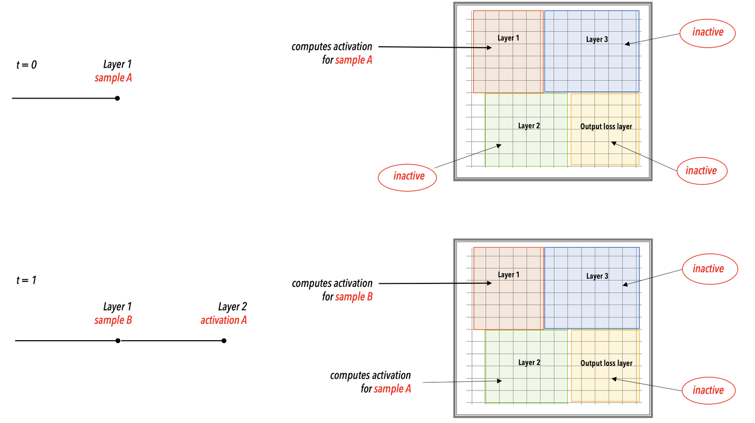
Fig. 9 Layer pipeline execution. In the layer pipelined execution, there is an initial latency period after which all the layers of the network enter a steady state of active execution. In this illustration, the network enters the steady state of execution at step 3 and thereafter.#
In the user node,
As loss values are computed on the WSE, they are streamed to the user node.
At specified intervals, all the weights can be downloaded to the user node to save checkpoints.
Differences between layer pipelined mode and weight streaming execution modes#
In weight streaming (WS), activations and gradients for one minibatch reside on the wafer at any given time. In layer pipelined (LP), there are several minibatches in flight on the wafer, and activations for all of them are resident.
In LP, all weights reside on the wafer and are updated there. In WS, weights reside in the MemoryX service. Weights are streamed into the wafer one layer at a time where the activations (forward prop) or gradients (backprop) interact with them there. Weights are updated in the MemoryX service, after aggregated gradients reach it via SwarmX .
In LP, weight gradients are used to update weights in situ, on the wafer, and can then be deleted. In WS, the weight gradients are sent via SwarmX for aggregation and then to MemoryX for weight updates.