Cerebras Execution Modes
On This Page
Cerebras Execution Modes
Basic concept
On the Cerebras Wafer Scale Engine (WSE) you can run neural networks of sizes ranging from extremely large, such as a GPT-3 model (with ~1 billion parameters) or a smaller sized model.
The execution mode refers to how the Cerebras runtime loads your neural network model onto the Cerebras Wafer Scale Engine (WSE). Two execution modes are supported:
Layer pipelined: In this mode all the layers of the network are loaded altogether onto the Cerebras WSE. This mode is selected for neural network models of a standard size, or even smaller.
Weight streaming: In this mode one layer of the neural network model is loaded at a time. This layer-by-layer mode is used to run extremely large models.
The rest of this section provides a high-level understanding of these two execution modes, using a simple FC-MNIST network as an example.
Example neural network
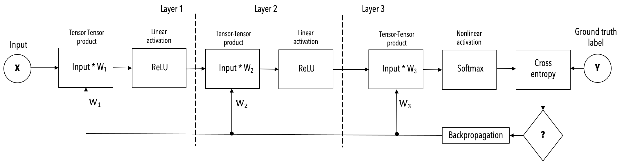
The simplified example, shown below, of a 3-layer FC-MNIST network is used in the following description of the two execution modes.
Layer pipelined mode
The layer pipelined execution mode works like this:
The Cerebras compiler maps each layer of the network onto a part of the Cerebras WSE. The compiler makes use of the parallelism in the model to perform such optimal mapping.
During the runtime, this entire network is loaded onto the Cerebras wafer at once.
Training data is streamed into the WSE continuously.
Weights are updated on the WSE and remain in the memory on the WSE within the layer to which they belong.
Activations also remain in the memory on the WSE and are passed on from layer to layer.
See the following simplified mathematical representation of our example network showing color-coded layers and the activations flowing from one layer to the next layer:
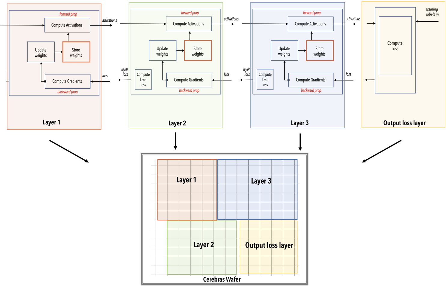
Layer pipeline mapping
The following diagram shows how our example network is mapped by the compiler onto the WSE. Notice that all the layers are mapped at once onto the WSE.
Note
The color-coded parts of the WSE, as shown below, onto which the network is mapped is only an example illustration. The compiler will place the network on any part of the network that results in optimal execution.
Layer pipeline execution
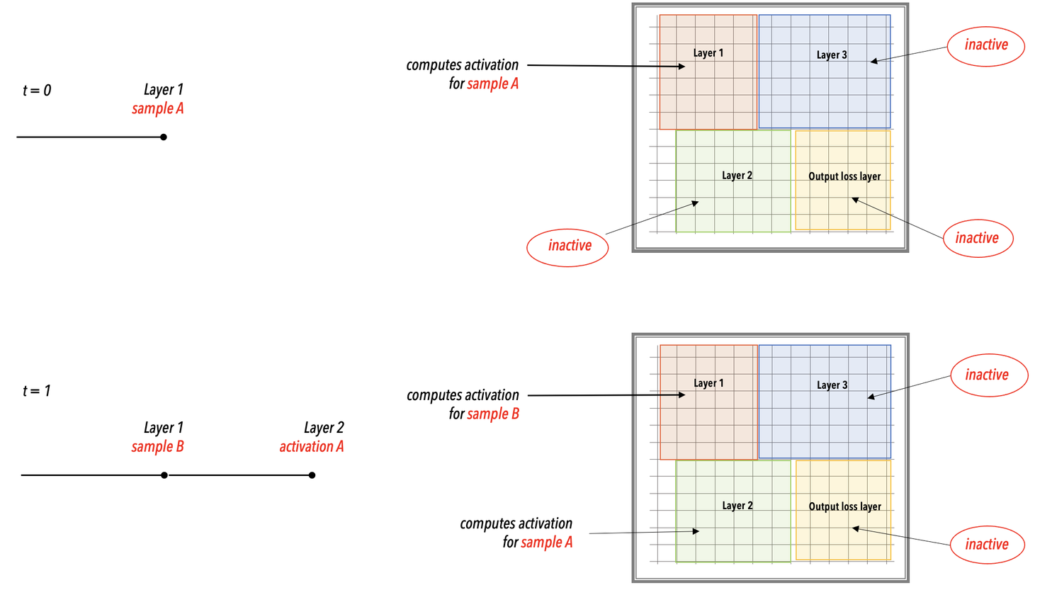
During the runtime, as the training samples are streamed into the WSE, the network will execute layer by layer in a layer pipelined manner. See the following example showing the incoming training samples A, B, C and D and forward propagation computation.
Note
In the layer pipelined execution, there is an initial latency period after which all the layers of the network enter a steady state of active execution. In the illustration below, the network enters the steady state of execution at t=3 and thereafter.
Weight streaming
The weight streaming execution mode is used for extremely large neural network models and for networks with very large input sizes. In the weight streaming execution mode the network is loaded layer by layer onto the WSE. Moreover, the weight streaming mode differs from the layer pipelined mode in the way the activations, the weights, and the gradients are handled. See the following:
Differences from layer pipeline model
This section describes how the weight streaming computation model differs from that of the layer pipeline mode.
Going from the layer pipelined computation to the weight streaming computation, the following are the key changes:
From streaming activations (in layer pipelined) → Store and read activations on the wafer (in weight streaming).
From storing gradients on the wafer → Stream gradients off the wafer.
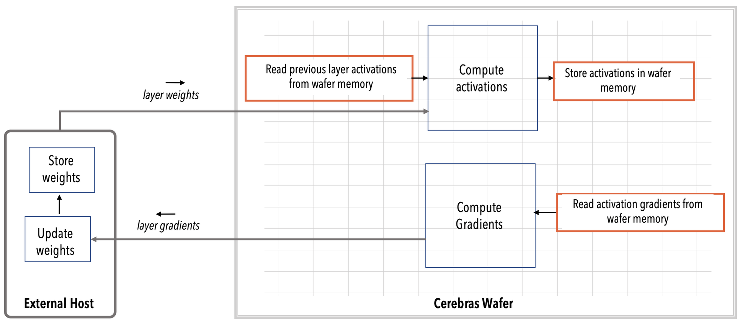
From store and read weights on the wafer → Stream weights off the wafer, update weights off the wafer by making use of the streamed gradients, store the weights off the wafer and stream the updated weights back into the wafer. See the following diagrams.
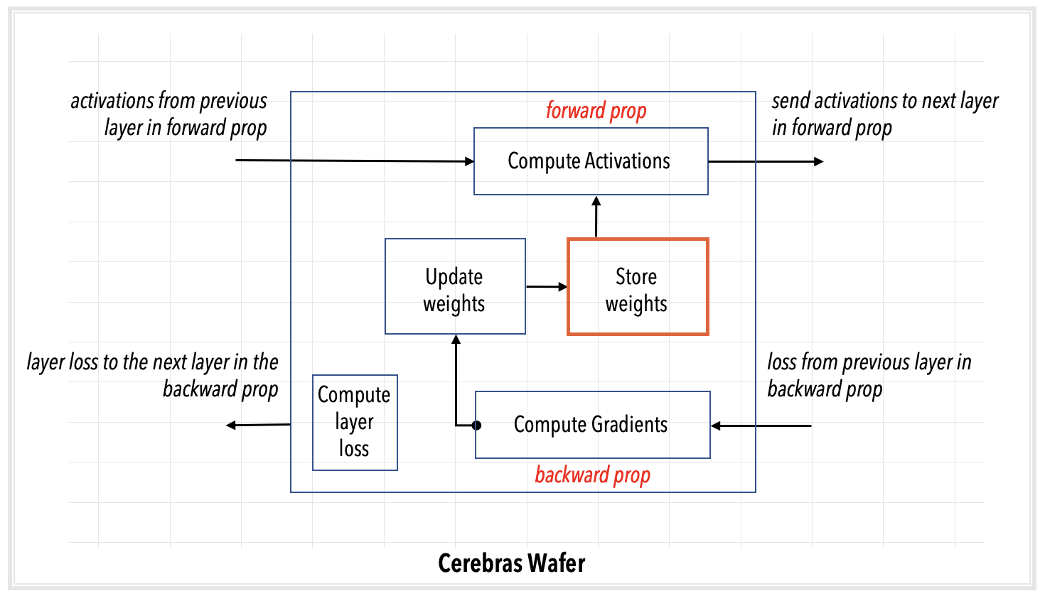
Layer pipelined computation
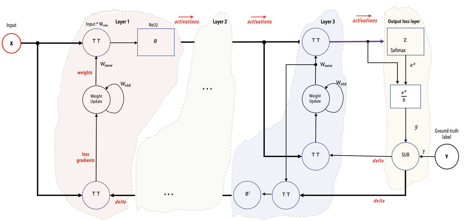
Weight streaming computation
Weight streaming execution
During the runtime, each layer is loaded onto the WSE at a single time, as shown in the following simplified diagram. A single layer is executed each time instance. For each layer, the gradients and weights are streamed off the wafer to the external host for storage and weight update computations, as described above.
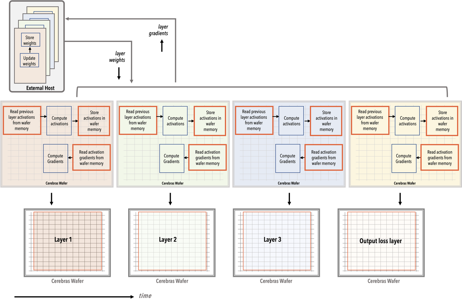
Forward propagation
For the FC-MNIST example, the forward propagation computation in weight streaming mode proceeds as follows:
The layer 1 is loaded onto the WSE first. The training data input and layer 1 weights are streamed into the WSE from the external host.
The entire WSE performs the layer 1 forward computations.
The computed activations for layer 1 remain in the WSE memory.
Next, the layer 2 is loaded onto the WSE, and the layer 2 weights are streamed from the external host into the WSE.
The entire WSE performs the layer 2 forward computations using the layer 1 activations that are in the WSE memory.
The computed activations for layer 2 remain in the WSE memory, to be used for layer 3 forward compute.
In this manner the forward compute for each layer is performed by using the stored computed activations of the prior layer. The computed activations of the current layer, in turn, are stored on the WSE memory to be used by the next layer that is loaded.
At the final output loss computation layer, the ground truth labels from the training data are used to compute the network loss delta. This loss delta is used to compute the gradients during the backward pass.
See the WSE snapshots below showing each forward compute layer for training data input sample 1.
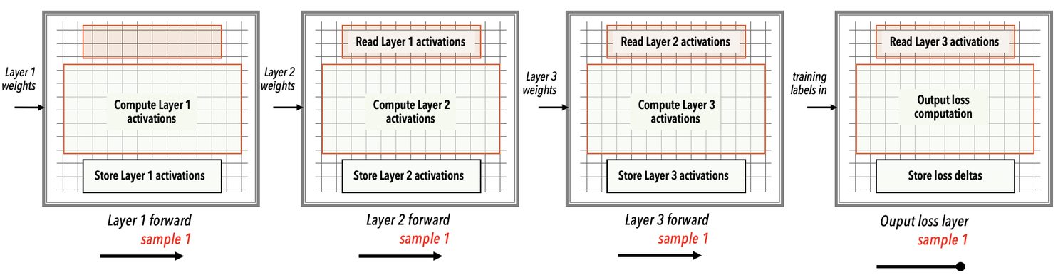
Note
In the above WSE snapshots, the rectangles only indicate the key operations that are performed on the WSE–these rectangles as shown do not represent how these operations are distributed on the WSE.
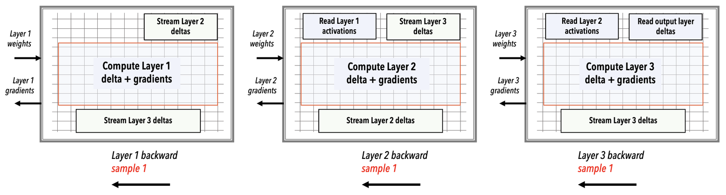
Backward propagation
Similarly, in the backward pass:
The layer 3 weights are streamed in and the WSE performs the gradient and delta computations for the layer 3.
The above-computed layer 3 gradients are streamed out of wafer to the external host. The external host uses these gradients to update the layer weights.
Next, the layer 2 weights are streamed in and the WSE similarly performs the gradient and delta computations for the layer 2. The layer 2 gradients are then streamed out of the wafer to the external host where weight updates occur.
The backward pass continues in this manner until layer 1 gradients are streamed out to the external host where the weights are updated and the next forward pass begins with the updated weights.